Analyse hsa-miR-124a-3p transfection time-course
Note
In order to do this analysis you have to be in the tests directory of GEOparse.
In the paper Systematic identification of microRNA functions by combining target prediction and expression profiling Wang and Wang provided a series of microarrays from 7 time-points after miR-124a transfection. The series can be found in GEO under the GSE6207 accession. We use this series to demonstrate general principles of GEOparse.
Warning
Mind that this tutorial is not abut how to properly calculate log fold changes - the approach undertaken here is simplistic.
We start with the imports:
import GEOparse
import pandas as pd
import pylab as pl
import seaborn as sns
pl.rcParams['figure.figsize'] = (14, 10)
pl.rcParams['ytick.labelsize'] = 12
pl.rcParams['xtick.labelsize'] = 11
pl.rcParams['axes.labelsize'] = 23
pl.rcParams['legend.fontsize'] = 20
sns.set_style('ticks')
c1, c2, c3, c4 = sns.color_palette("Set1", 4)
Now we select the GSMs that are controls. See below on how to generate names of control samples directly from the phenotype data of GSE.
controls = ['GSM143386',
            'GSM143388',
            'GSM143390',
            'GSM143392',
            'GSM143394',
            'GSM143396',
            'GSM143398']
Using GEOparse we can download experiments and look into the data:
gse = GEOparse.get_GEO("GSE6207")
File already exist: using local version.
Parsing ./GSE6207.soft.gz:
 - DATABASE : GeoMiame
 - SERIES : GSE6207
 - PLATFORM : GPL570
 - SAMPLE : GSM143385
 - SAMPLE : GSM143386
 - SAMPLE : GSM143387
 - SAMPLE : GSM143388
 - SAMPLE : GSM143389
 - SAMPLE : GSM143390
 - SAMPLE : GSM143391
 - SAMPLE : GSM143392
 - SAMPLE : GSM143393
 - SAMPLE : GSM143394
 - SAMPLE : GSM143395
 - SAMPLE : GSM143396
 - SAMPLE : GSM143397
 - SAMPLE : GSM143398
The GPL we are interested:
gse.gpls['GPL570'].columns
| description | |
|---|---|
| ID | Affymetrix Probe Set ID LINK_PRE:"https://www.... |
| GB_ACC | GenBank Accession Number LINK_PRE:"http://www.... |
| SPOT_ID | identifies controls |
| Species Scientific Name | The genus and species of the organism represen... |
| Annotation Date | The date that the annotations for this probe a... |
| Sequence Type | |
| Sequence Source | The database from which the sequence used to d... |
| Target Description | |
| Representative Public ID | The accession number of a representative seque... |
| Gene Title | Title of Gene represented by the probe set. |
| Gene Symbol | A gene symbol, when one is available (from Uni... |
| ENTREZ_GENE_ID | Entrez Gene Database UID LINK_PRE:"http://www.... |
| RefSeq Transcript ID | References to multiple sequences in RefSeq. Th... |
| Gene Ontology Biological Process | Gene Ontology Consortium Biological Process de... |
| Gene Ontology Cellular Component | Gene Ontology Consortium Cellular Component de... |
| Gene Ontology Molecular Function | Gene Ontology Consortium Molecular Function de... |
And the columns that are available for exemplary GSM:
gse.gsms["GSM143385"].columns
| description | |
|---|---|
| ID_REF | Affymetrix probe set ID |
| VALUE | RMA normalized Signal intensity (log2 transfor... |
We take the opportunity and check if everything is OK with the control samples. For this we just use simple histogram. To obtain table with each GSM as column, ID_REF as index and VALUE in each cell we use pivot_samples method from GSE object (we restrict the columns to the controls):
pivoted_control_samples = gse.pivot_samples('VALUE')[controls]
pivoted_control_samples.head()
| name | GSM143386 | GSM143388 | GSM143390 | GSM143392 | GSM143394 | GSM143396 | GSM143398 |
|---|---|---|---|---|---|---|---|
| ID_REF | |||||||
| 1007_s_at | 9.373339 | 9.316689 | 9.405605 | 9.332526 | 9.351024 | 9.245251 | 9.423234 |
| 1053_at | 8.453839 | 8.440368 | 8.435023 | 8.411635 | 8.373939 | 8.082178 | 7.652785 |
| 117_at | 5.878466 | 5.928938 | 5.969288 | 5.984232 | 5.882761 | 5.939399 | 6.027338 |
| 121_at | 9.131430 | 9.298601 | 9.176132 | 9.249977 | 9.149849 | 9.250952 | 9.352397 |
| 1255_g_at | 3.778179 | 3.861210 | 3.740103 | 3.798814 | 3.761673 | 3.790185 | 3.895462 |
And we plot:
pivoted_control_samples.hist()
sns.despine(offset=10, trim=True)
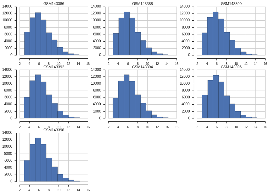
Next we would like to filter out probes that are not expressed. The gene is expressed (in definition here) when its average log2 intensity in control samples is above 0.25 quantile. I.e. we filter out worst 25% genes.
pivoted_control_samples_average = pivoted_control_samples.median(axis=1)
print("Number of probes before filtering: ", len(pivoted_control_samples_average))
Number of probes before filtering: 54675
expression_threshold = pivoted_control_samples_average.quantile(0.25)
expressed_probes = pivoted_control_samples_average[pivoted_control_samples_average >= expression_threshold].index.tolist()
print("Number of probes above threshold: ", len(expressed_probes))
Number of probes above threshold: 41006
We can see that the filtering succeeded. Now we can pivot all the samples and filter out probes that are not expressed:
samples = gse.pivot_samples("VALUE").ix[expressed_probes]
The most important thing is to calculate log fold changes. What we have to do is for each time-point identify control and transfected sample and subtract the VALUES (they are provided as log2 transformed already, we subtract transfection from the control).
In order to identify control and transfection samples we will take a look into phenotype data and based on it we decide how to split samples:
print gse.phenotype_data[["title", "source_name_ch1"]]
                                                 title  source_name_ch1
GSM143385             miR-124 transfection for 4 hours  HepG2 cell line
GSM143386    negative control transfection for 4 hours  HepG2 cell line
GSM143387             miR-124 transfection for 8 hours  HepG2 cell line
GSM143388    negative control transfection for 8 hours  HepG2 cell line
GSM143389            miR-124 transfection for 16 hours  HepG2 cell line
GSM143390   negative control transfection for 16 hours  HepG2 cell line
GSM143391            miR-124 transfection for 24 hours  HepG2 cell line
GSM143392   negative control transfection for 24 hours  HepG2 cell line
GSM143393            miR-124 transfection for 32 hours  HepG2 cell line
GSM143394   negative control transfection for 32 hours  HepG2 cell line
GSM143395            miR-124 transfection for 72 hours  HepG2 cell line
GSM143396   negative control transfection for 72 hours  HepG2 cell line
GSM143397           miR-124 transfection for 120 hours  HepG2 cell line
GSM143398  negative control transfection for 120 hours  HepG2 cell line
We can see that based on the title of the experiment we can get all the information that we need:
experiments = {}
for i, (idx, row) in enumerate(gse.phenotype_data.iterrows()):
    tmp = {}
    tmp["Experiment"] = idx
    tmp["Type"] = "control" if "control" in row["title"] else "transfection"
    tmp["Time"] = re.search(r"for (\d+ hours)", row["title"]).group(1)
    experiments[i] = tmp
experiments = pd.DataFrame(experiments).T
print experiments
   Experiment       Time          Type
0   GSM143385    4 hours  transfection
1   GSM143386    4 hours       control
2   GSM143387    8 hours  transfection
3   GSM143388    8 hours       control
4   GSM143389   16 hours  transfection
5   GSM143390   16 hours       control
6   GSM143391   24 hours  transfection
7   GSM143392   24 hours       control
8   GSM143393   32 hours  transfection
9   GSM143394   32 hours       control
10  GSM143395   72 hours  transfection
11  GSM143396   72 hours       control
12  GSM143397  120 hours  transfection
13  GSM143398  120 hours       control
In the end we create new DataFrame with LFCs:
lfc_results = {}
sequence = ['4 hours',
             '8 hours',
             '16 hours',
             '24 hours',
             '32 hours',
             '72 hours',
             '120 hours']
for time, group in experiments.groupby("Time"):
    print(time)
    control_name = group[group.Type == "control"].Experiment.iloc[0]
    transfection_name = group[group.Type == "transfection"].Experiment.iloc[0]
    lfc_results[time] = (samples[transfection_name] - samples[control_name]).to_dict()
lfc_results = pd.DataFrame(lfc_results)[sequence]
120 hours
16 hours
24 hours
32 hours
4 hours
72 hours
8 hours
Let’s look at the data sorted by 24-hours time-point:
lfc_results.sort("24 hours").head()
| 4 hours | 8 hours | 16 hours | 24 hours | 32 hours | 72 hours | 120 hours | |
|---|---|---|---|---|---|---|---|
| 214149_s_at | 0.695643 | -0.951014 | -1.768543 | -3.326683 | -2.954085 | -3.121960 | -1.235596 |
| 214835_s_at | -0.120661 | -1.282502 | -2.540301 | -3.238786 | -3.183429 | -3.284111 | -1.901547 |
| 212459_x_at | 0.010564 | -1.092724 | -2.235531 | -3.203148 | -3.115878 | -3.008434 | -1.706501 |
| 201171_at | 0.958699 | -1.757044 | -1.571311 | -3.173688 | -3.061849 | -2.672462 | -1.456556 |
| 215446_s_at | -0.086179 | -0.408025 | -1.550514 | -3.083213 | -3.024972 | -4.374527 | -2.581921 |
We are interested in the gene expression changes upon transfection. Thus, we have to annotate each probe with ENTREZ gene ID, remove probes without ENTREZ or with multiple assignments. Although this strategy might not be optimal, after this we average the LFC for each gene over probes.
# annotate with GPL
lfc_result_annotated = lfc_results.reset_index().merge(gse.gpls['GPL570'].table[["ID", "ENTREZ_GENE_ID"]],
                                left_on='index', right_on="ID").set_index('index')
del lfc_result_annotated["ID"]
# remove probes without ENTREZ
lfc_result_annotated = lfc_result_annotated.dropna(subset=["ENTREZ_GENE_ID"])
# remove probes with more than one gene assigned
lfc_result_annotated = lfc_result_annotated[~lfc_result_annotated.ENTREZ_GENE_ID.str.contains("///")]
# for each gene average LFC over probes
lfc_result_annotated = lfc_result_annotated.groupby("ENTREZ_GENE_ID").median()
We can now look at the data:
lfc_result_annotated.sort("24 hours").head()
| 4 hours | 8 hours | 16 hours | 24 hours | 32 hours | 72 hours | 120 hours | |
|---|---|---|---|---|---|---|---|
| ENTREZ_GENE_ID | |||||||
| 8801 | -0.027313 | -1.130051 | -2.189180 | -3.085749 | -2.917788 | -2.993609 | -1.700850 |
| 8992 | 0.342758 | -0.884020 | -1.928357 | -3.017827 | -3.024406 | -2.991851 | -1.160622 |
| 9341 | -0.178168 | -0.591781 | -1.708289 | -2.743563 | -2.873147 | -2.839508 | -1.091627 |
| 201965 | -0.109980 | -0.843801 | -1.910224 | -2.736311 | -2.503068 | -2.526326 | -1.081906 |
| 84803 | -0.051439 | -0.780564 | -1.979405 | -2.513718 | -3.123384 | -2.506667 | -1.035104 |
At that point our job is basicaly done. However, we might want to check if the experiments worked out at all. To do this we will use hsa-miR-124a-3p targets predicted by MIRZA-G algorithm. The targets should be downregulated. First we read MIRZA-G results:
header = ["GeneID", "miRNA", "Total score without conservation", "Total score with conservation"]
miR124_targets = pd.read_table("seed-mirza-g_all_mirnas_per_gene_scores_miR_124a.tab", names=header)
miR124_targets.head()
| GeneID | miRNA | Total score without conservation | Total score with conservation | |
|---|---|---|---|---|
| 0 | 55119 | hsa-miR-124-3p | 0.387844 | 0.691904 |
| 1 | 538 | hsa-miR-124-3p | 0.243814 | 0.387032 |
| 2 | 57602 | hsa-miR-124-3p | 0.128944 | NaN |
| 3 | 3267 | hsa-miR-124-3p | 0.405515 | 0.371705 |
| 4 | 55752 | hsa-miR-124-3p | 0.411628 | 0.373977 |
We shall extract targets as a simple list of strings:
miR124_targets_list = map(str, miR124_targets.GeneID.tolist())
print("Number of targets:", len(miR124_targets_list))
Number of targets: 2311
As can be seen there is a lot of targets (genes that posses a seed match in their 3’UTRs). We will use all of them. As first stem we will annotate genes if they are targets or not and add this information as a column to DataFrame:
lfc_result_annotated["Is miR-124a target"] = [i in miR124_targets_list for i in lfc_result_annotated.index]
cols_to_plot = [i for i in lfc_result_annotated.columns if "hour" in i]
In the end we can plot the results:
a = sns.pointplot(data=lfc_result_annotated[lfc_result_annotated["Is miR-124a target"]][cols_to_plot],
                   color=c2,
                   label="miR-124a target")
b = sns.pointplot(data=lfc_result_annotated[~lfc_result_annotated["Is miR-124a target"]][cols_to_plot],
             color=c1,
             label="No miR-124a target")
sns.despine()
pl.legend([pl.mpl.patches.Patch(color=c2), pl.mpl.patches.Patch(color=c1)],
          ["miR-124a target", "No miR-124a target"], frameon=True, loc='lower left')
pl.xlabel("Time after transfection")
pl.ylabel("Median log2 fold change")
<matplotlib.text.Text at 0x7fe66c094410>
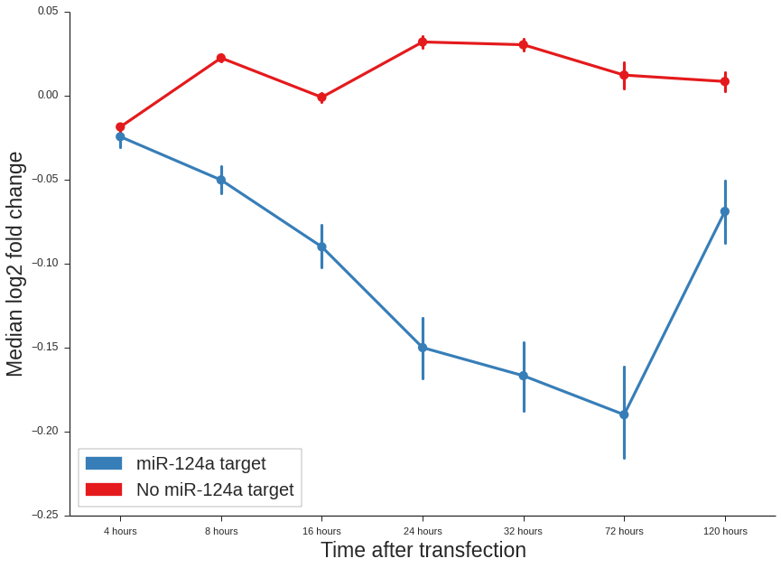
As can be seen the targets of hsa-miR-124a-3p behaves in the expected way. With each time-point their downregulation is stronger up the 72 hours. After 120 hours the transfection is probably lost. This means that the experiments worked out.